I wrote a blog post about how to implement your own (operator overloading based) automatic differentiation (AD) in one day (actually 3 hrs) last year. AD looks like magic sometimes, but I’m going to talk about some black magic this time: the source
to source automatic differentiation. I wrote this during JuliaCon 2019 hackthon with help from Mike Innes.
It turns out that writing a blog post takes longer than writing a source to source AD ;-). This is basically just simple version of Zygote.
I wrap this thing as a very simple package here, if you want to look at more detailed implementation: YASSAD.jl.
If you have used operator overloading based AD like PyTorch, Flux/Tracker, AutoGrad, you may find they have some limitations:
- A
Tensortype orVariabletype provided by the package has to be used for tracing the function calls - They cannot handle control flows in general, even in some cases, some workarounds can be taken
However, programming without control flow is not programming! And it is usually very annoying to rewrite a lot code with tracked types. If we want to have a framework for Differentiable Programming as what people like Yan LeCun has been proposing, we need to solve these two problems above.
In fact, these problems are quite straight forward to solve in source to source automatic differentiation, since we basically know everything happens. I will implement a very simple source to source AD without handling control flows, you can also check the complete implementation as Zygote.jl.
But before we start, let’s review some basic knowledge.
Basics
The compilation process of Julia language
I will briefly introduce how Julia program is compiled and run in this section:
- all the code are just strings
- the Julia parser will parse the strings first to get an Abstract Syntax Tree (AST)
- some of the nodes in this AST are macros, macros are like compiled time functions on expressions, the compiler will expand the macros. Then we get an expanded version of AST, which do not have any macros. You can inspect the results with
@macroexpand. - Now, we will lower the AST, get rid of syntax sugars and represent them in Static Single Assignment Form (SSA), you can get it with
@code_lowered, and you can modify this process with Juliamacros. - When function call happens, we use the function signature to dispatch the function to a certain method, and start doing type inference. You can modify this process with
@generatedfunctions, and check the results with@code_typed. - The compiler will then generate the llvm IR. You can inspect them with
@code_llvm - After we have llvm IR, Julia will use llvm to generate native code to actually exectute this function.
- By executing the function, we will meet another function call, so we go back to step 5
I steal a diagram from JuliaCon 2018 to demonstrate this process:
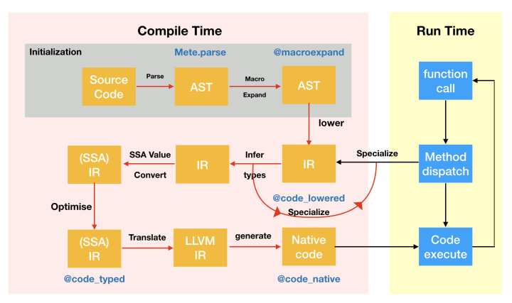
As you can see. Julia is not a static compiled language, and it uses function as boundary of compilation.
SSA Form IR
A complete introduction of SSA can be a book. But to implement your own source
to source AD only require three simple concept:
- all the variable will only be assigned once
- most variable comes from function calls
- all the control flows become branches
If you have read my last post, I believe you have understand what is computation graph, but now let’s look at this diagram again: what is this computation graph exactly?
While doing the automatic differentiation, we represent the process of computation as a diagram. Each node is an operator with a intermediate value. And each operator also have an adjoint operator which will be used in backward pass. Which means each variable
in each node will only be assigned once. This is just a simple version of SSA Form right?
The gradient can be then considered as an adjoint program of the original program. And the only thing we need to do is to generate the adjoint program. In fact, this is often called Wengert list, tape or graph as described in Zygote’s paper: Don’t Unroll Adjoint. Thus we can directly use the SSA form as our computational graph. Moreover, since in Julia the SSA form IR is lowered, it also means we only need to defined a few primitive routines instead of defining a lot operators.
Since the backward pass is just an adjoint of the original program, we can just write it as a closure
1 | function forward(::typeof(your_function), xs...) |
The advantage of defining this as closure is that we can let the compiler itself handle shared variable between the adjoint program
and the original program instead of managing it ourselves (like what we do in my last post). We call these closures pullbacks.
So given a function like the following
1 | function foo(x) |
If we do this manually, we only need to define a forward function
1 | function forward(::typeof(foo), x) |
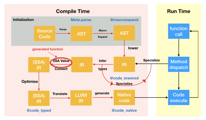
In general, an adjoint program without control flow is just applying these pullbacks generated by their forward function in reversed order. But how do we do this automatically? Someone may say: let’s use macros! Err, we can do that. But our goal is to differentiate arbitrary function defined by someone else, so things can be composable. This is not what we want. Instead, we can tweak the IR, the generated functions in Julia can not only return a modified AST from type information, it can also return the IR.
The generated function can be declared with a @generated macro
1 | function foo(a, b, c) |
It looks like a function as well, but the difference is that inside the function, the value of each function argument a, b, c
is their type since we do not have their values during compile time.
In order to manipulate the IR, we need some tools. Fortunately, there are some in IRTools, we will use this package to generate the IR code.
First, we can use @code_ir to get the IR object processed by IRTools. Its type is IR. The difference between the one you get from @code_lowered is that this will not store the argument name, all the variables are represented by numbers, and there are some useful function implemented for this type.
1 | julia> foo(1.0) |
In this form, each line of code is binded to a variable, we call the right hand statement, and left hand variable. You use a dict-like interface to use this object, e.g
1 | julia> using IRTools: var |
It will return a statement object, which stores the expression of this statement, the inferred type (since we are using the IR before type inference, this is Any). For simplicity, we will not use typed IR in this post (since in principal, their implementations are similar). The last number is the line number.
What is the first number 1 in the whole block? It means code block, in SSA form we use this to represent branches, e.g
1 | julia> function foo(x) |
ifelse is just branch statement in lowered SSA form, and in fact, for loops are similar. Julia’s for loop is just a syntax sugar of iterate function. As long as we can differentiate through br, we will be able to differentiate through control flows.
1 | julia> function foo(x) |
So how do we get the IR? In order to get the IR, we need to know which method is dispatched for this generic function. Each generic
function in Julia has a method table, you can use the type signature of the function call to get this method, e.g when you call foo(1.0), Julia will generate Tuple{typeof(foo), Float64} to call the related method. We can get the meta information of this method by providing the IRTools.meta function with this type signature
1 | julia> IRTools.IR(m) |
And we can manipulate this IR with functions like push!:
1 | julia> push!(ir, :(1+1)) |
IRTools will add the variable name for you automatically here. Similarly, we can use insert! to insert a statement before the 4th variable:
1 | julia> using IRTools: var |
Or we can insert a statement after the 4th variable:
1 | julia> using IRTools: insertafter! |
With these tools, we can now do the transformation of forward pass. Our goal is to replace each function call with the function call to forward function and then collect all the pullbacks returned by forward function to generate a closure. But wait! I didn’t mention closure, what is the closure in SSA IR? Let’s consider this later, and implement the transformation of forward part first.
Let’s take a statement and have a look
1 | julia> dump(ir[var(3)]) |
In fact, we only need to check whether the signature of its expression is call. We can use the Pipe object in IRTools to do the transformation, the transformation results are stored in its member to.
1 | julia> IRTools.Pipe(ir).to |
Implementation
Forward Transformation
We name this function as register since it has similar functionality as our old register function in my last post. The only difference is: you don’t need to write this register function manually for each operator now! We are going to do this automatically.
Warning: since I’m doing this demo in REPL, I use Main module directly, if you put the code in your own module, replace it with your module name.
1 | function register(ir) |
I’ll explain what I do here: first since we are generating the IR for the forward function, we have an extra argument now
1 | forward(f, args...) |
Thus, I added one argument at the beginning of this function’s IR.
Then, we need to iterate through all the variables and statements, if the statement is a function call then we replace it with the call
to forward function. Remember to keep the line number here, since we still want some error message. Since the returned value of forward is a tuple of actually forward evaluation and the pullback, to get the correct result we need to index this tuple, and replace
the original variable with the new one. The xgetindex here is a convenient function that generates the expression of getindex
1 | xgetindex(x, i...) = xcall(Base, :getindex, x, i...) |
Let’s see what we get
1 | julia> register(ir) |
Nice! We change the function call to forward now!
Now, it’s time to consider the closure problem. Yes, in this lowered form, we don’t have closures. But we can instead store them in a callable object!
1 | struct Pullback{S, T} |
This object will also store the function signature, so when we call pullback, we can look up the IR of the original call to generate the IR of this pullback. The member data here will store a Tuple of all pullbacks with the order of their forward call. In order to construct the Pullback we need the signature of our function call, so we need to revise our implementation as following.
1 | function register(ir, F) |
In order to store the pullbacks, we need to get the pullback from the tuple returned by forward and allocate a list to record all pullbacks.
Here xtuple is similar to xgetindex, it is used to generate the expression of constructing a tuple.
1 | xtuple(xs...) = xcall(Core, :tuple, xs...) |
Let’s pack the pullback and the original returned value as a tuple together, and return it!
1 | function register(ir, F) |
The return statement is actually a simple branch, it is the last branch of the last statement of the last code block.
OK, let’s see what we get now
1 | julia> register(ir, Tuple{typeof(foo), Float64}) |
Now let’s implement the forward function
1 | function forward(f, xs...) |
We will get the meta first, if the meta is nothing, it means this method doesn’t exist, so we just stop here. If we have the meta, then
we can get the IR from it and put it to register
1 | function forward(f, xs...) |
However, the object frw has type IR instead of CodeInfo, to generate the CodeInfo for Julia compiler, we need to put argument names back with
1 | argnames!(m, Symbol("#self#"), :f, :xs) |
And since the second argument of our forward function is a vararg, we need to tag it to let our compiler know, so the compiler will not feed the first function call with a Tuple.
1 | frw = varargs!(m, frw, 2) |
In the end, our forward function will looks like
1 | function forward(f, xs...) |
Let’s see what we got now
1 | julia> forward(foo, 1.0) |
If you try to actually run this, there will be some error unfortunately
1 | julia> forward(foo, 1.0) |
This is because the forward will be recursively called, which also means we only need to define the inner most (primitive) operators by overloading the forward functions, e.g we can overload the * operator in this case
1 | julia> forward(::typeof(*), a::Real, b::Real) = a * b, Δ->(Δ*b, a*Δ) |
Backward Transformation
But this pullback is not callable yet. Let’s generate the IR for pullback. Similarly, we can define
1 | function (::Pullback{S})(delta) where S |
Because the backward pass is called separately, we don’t have the forward IR anymore, unfortunately we need to call register again here, but no worries, this will only happen once during compile time. Before we generate the IR for adjoint program, we also need to know which variable has pullback, thus instead of using a list, we need a dict to store this, and return it to pullback. Therefore, we need to revise our register as following
1 | function register(ir, F) |
since the adjoint program has the reversed order with the original IR, we will not use Pipe here, we can create an empty IR object,
and add two argument to it here, one is the Pullback object itself, the other is the input gradient of the backward pass (pullback).
1 | adj = empty(ir) |
First, let’s get our pullbacks. The getfield function I call here is the lowered form of syntax sugar . for getting members, this is equivalent to self.data.
1 | pullbacks = pushfirst!(adj, xcall(:getfield, self, QuoteNode(:data))) |
Then let’s iterate the all the variables in reversed order
1 | vars = keys(ir) |
if this variable exists in our dict of pullbacks, we get it and call it with this variable. However, there is a problem of this implementation, if one variable has multiple gradient, we need to accumulate them together, thus we need to record these variables’
gradietns as well.
1 | grads = Dict() |
Then we can implement two method of grad:
1 | grad(x, x̄) = push!(get!(grads, x, []), x̄) |
Store the gradient x̄ in the list of x in grads.
1 | grad(x) = xaccum(adj, get(grads, x, [])...) |
Return the accumulated variable of all gradients.
The xaccum is the same as previous xgetindex, but the builtin accumulate function in Julia is defined on arrays, we need one to accumulate variant variables, let’s do it ourselves
1 | xaccum(ir) = nothing |
In the end, the pullback will return each input variable’s gradient of the original program. Which means it always has
the same number of gradients as input variables. But our forward function has one extra variable which is the function,
we will return its gradient as well, in most cases, it is nothing, but if it is a closure, or a callable object, it may
not be nothing.
So, in the end, our adjoint function looks like
1 | function adjoint(ir, pbs) |
Contextual Dispatch
Reviewing what we just implemented above, we can find we were actually just dispatching functions based on their context instead of
their signature (since the signature is used to dispatch the function themselves). The Julia community actually implements something
more general: the Cassette.jl. Cassette can dispatch function based on a context, and it also contains an implementation of AD as well: Cassette/test. With these mechanism, and the dynamic feature of Julia, we are not only able to implement source to source AD, we can also have
- Sparsity Detection
- SPMD transformation
- Intermediate Variable Optimization
- Debugger: MagneticReadHead
- Unified Interface of CUDAnative
Conclusion
Let’s try this with matrix multiplication + matrix trace, which is the same with what we do in our last post!
Look! we can use the builtin types directly!
1 | using LinearAlgebra |
The performance is similar to the manual implementation as well (in fact it should be the same)
The manual version is:
1 | julia> bench_tr_mul_base($(rand(30, 30)), $(rand(30, 30))) |
the generated version:
1 | julia> tr_mul($A, $B) |
Now we have implemented a very simple source to source automatic differentiation, but we didn’t handle control flow here. A more
complete implementation can be find in Zygote.jl/compiler, it can differentiate through almost everything, including: self defined types, control flows, foreign function calls (e.g you can differentiate PyTorch functions!), and in-place function (mutation support). This also includes part of our quantum algorithm design framework Yao.jl with some custom primitives.
Our implementation here only costs 132 lines of code in Julia. Even the complete implementation’s compiler only costs 495 lines of code. It is possible to finish in one or a few days!