Half Integer

How hard is it to build your own top performance quantum circuit simulator? Does it really needs thousands of lines of code to implement it?
At least in Julia language, you don’t! We can easily achieve top performance via a few hundreds of code while supporting
CUDA and symbolic calculation.

Like my previous blog posts, you can do it in ONE DAY as well. I’ll introduce how to do this with Julia language while going
through some common tricks for high performance computing in Julia language. I won’t talk much about the Julia language itself
or it will be a very long blog post, thus if you want to follow this blog post but you don’t know how to use the Julia programming
language yet, I would suggest you to checkout materials here first.

Background

Quantum computing has been a popular research topic in recent years. And building simulators can be useful for related research. I’m not going to give you a full introduction of what is quantum computing in this blog post, but I find you this nice tutorial from Microsoft if you are
interested in knowing what is the quantum computing. And you don’t really need to understand everything about quantum computing to follow this blog post - the emulator itself is just about special matrix-vector or matrix-matrix multiplication.

So to be simple, simulating quantum circuits, or to be more specific simulating how quantum circuits act on a quantum register, is about how to calculate large matrix-vector multiplication that scales exponentially. The most brute-force and accurate way of doing it via full amplitude simulation, which means we do this matrix-vector multiplication directly.

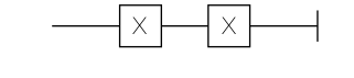
The vector contains the so-called quantum state and the matrices are quantum gate, which are usually small. The diagram of quantum circuits is a representation of these matrix multiplications. For example, the X gate is just a small matrix

$$
\begin{pmatrix}
0 & 1\\
1 & 0
\end{pmatrix}
$$

In theory, there is no way to simulate a general quantum circuit (more precisely, a universal gate set) efficiently, however, in practice, we could still do it within a rather small scale with some tricks that make use of the structure of the gates.

To know how to calculate a quantum circuit in the most naive way, we need to know two kinds of mathematical operations

Tensor Product/Kronecker Product, this is represented as two parallel lines in the quantum circuit diagram, e.g

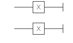
and by definition, this can be calculated by

$$
\begin{pmatrix}
a_{11} & a_{12} \\
a_{21} & a_{22}
\end{pmatrix} \otimes
\begin{pmatrix}
b_{11} & b_{12} \\
b_{21} & b_{22}
\end{pmatrix} =
\begin{pmatrix}
a_{11} \begin{pmatrix}
b_{11} & b_{12} \\
b_{21} & b_{22}
\end{pmatrix} & a_{12} \begin{pmatrix}
b_{11} & b_{12} \\
b_{21} & b_{22}
\end{pmatrix} \\
a_{21} \begin{pmatrix}
b_{11} & b_{12} \\
b_{21} & b_{22}
\end{pmatrix} & a_{22} \begin{pmatrix}
b_{11} & b_{12} \\
b_{21} & b_{22}
\end{pmatrix}
\end{pmatrix}
$$

Matrix Multiplication, this is the most basic linear algebra operation, I’ll skip introducing this. In quantum circuit diagram, this is represented by blocks connected by lines.

As a conclusion of this section, you can see simulating how pure quantum circuits act on a given quantum state is about how to implement some special type of matrix-vector multiplication
efficiently. If you know about BLAS (Basic Linear Algebra Subprograms), you will realize this kind of operations are only BLAS level 2 operations, which does not require any smart tiling
technique and are mainly limited by memory bandwidth.

So let’s do it!

Implementing general unitary gate

Thus the simplest way of simulating a quantum circuit is very straightforward: we can just make use of Julia’s builtin functions:
kron and *.

1
2
3
4
5

using LinearAlgebra
function naive_broutine!(r::AbstractVector, U::AbstractMatrix, loc::Int)
    n = Int(log2(length(r))) # get the number of qubits
    return kron(I(1<<(n-loc+1)), U), I(1<<loc)
end

However, this is obviously very inefficient:

1. we need to allocate a $2^n \times 2^n$ matrix every time we try to evaluate the gate.
2. the length of the vector can only be $2^n$, thus we should be able to calculate it faster with this knowledge.

I’ll start from the easiest thing: if we know an integer is $2^n$, it is straight forward to find out $n$ by the following method

1
2

log2i(x::Int64) = !signbit(x) ? (63 - leading_zeros(x)) : throw(ErrorException("nonnegative expected ($x)"))
log2i(x::UInt64) = 63 - leading_zeros(x)

this is because we already know how long our integer is in the program by looking at its type, thus simply minus the number of leading zeros would give us the answer.
But don’t forget to raise an error when it’s an signed integer type. We can make this work on any integer type by the following way

1
2
3
4
5
6
7
8
9
10

for N in [8, 16, 32, 64, 128]
    T = Symbol(:Int, N)
    UT = Symbol(:UInt, N)
    @eval begin
        log2i(x::$T) =
            !signbit(x) ? ($(N - 1) - leading_zeros(x)) :
            throw(ErrorException("nonnegative expected ($x)"))
        log2i(x::$UT) = $(N - 1) - leading_zeros(x)
    end
end

the command @eval here is called a macro in Julia programming language, it can be used to generate code. The above code generates the implementation of log2i for signed
and unsigned integer types from 8 bits to 128 bits.

Let’s now consider how to write the general unitary gate acting on given locations of qubits.

1
2

function broutine!(r::AbstractVector, U::AbstractMatrix, locs::NTuple{N, Int}) where N
end

this matrix will act on some certain qubits in the register, e.g given a 8x8 matrix we want it to act on the 1st, 4th and 5th qubit. Based on the implementation of X and Z we know this is about multiplying this matrix on the subspace of 1st, 4th and 5th qubit, which means we need to construct a set of new vectors whose indices iterate over the subspace of 0xx00x, 0xx01x, 0xx10x, 0xx11x etc. Thus the first thing we need to do is to find a generic way to iterate through the subspace of 0xx00x then by adding an offset such as 1<<1 to each index in this subspace, we can get the subspace of 0xx01x etc.

Iterate through the subspace

To iterate through the subspace, we could iterate through all indices in the subspace. For each index, we move each bit to its position in the whole space (from first bit to the last).
This will give us the first subspace which is 0xx00x.

Before we move on, I need to introduce the concept of binary masks: it is an integer that can help us “filter” out some binary values, e.g
we want to know if a given integer’s 4th and 5th bit, we can use a mask 0b11000, where its 4th and 5th bit are 1 the rest is 0, then we
can use an and operation get get the value. Given the location of bits, we can create a binary mask via the following bmask function

1
2
3
4
5
6
7
8

function bmask(itr)
    isempty(itr) && return 0
    ret = 0
    for b in itr
        ret += 1 << (b - 1)
    end
    return ret
end

where itr is some iterable. However there are quite a few cases that we don’t need to create it via a for-loop, so we can specialize this function
on the following types

1
2
3

function bmask(range::UnitRange{Int})
    ((1 << (range.stop - range.start + 1)) - 1) << (range.start - 1)
end

however, we maybe want to make the implementation more general for arbitrary integer types, so let’s use a type variable T!

1
2
3
4
5
6
7
8
9
10
11
12

function bmask(::Type{T}, itr) where {T<:Integer}
    isempty(itr) && return 0
    ret = zero(T)
    for b in itr
        ret += one(T) << (b - 1)
    end
    return ret
end

function bmask(::Type{T}, range::UnitRange{Int})::T where {T<:Integer}
    ((one(T) << (range.stop - range.start + 1)) - one(T)) << (range.start - 1)
end

However after we put a type variable as the first argument, it is not convenient when we just want to use Int64 anymore,
let’s create a few convenient methods then

1
2
3
4

bmask(args...) = bmask(Int, args...)
# this is for removing the infinity call of the later function
bmask(::Type{T}) where {T<:Integer} = zero(T)
bmask(::Type{T}, positions::Int...) where {T<:Integer} = bmask(T, positions)

The final implement would look like the following

1
2
3
4
5
6
7
8
9
10
11
12
13
14
15
16

bmask(args...) = bmask(Int, args...)
bmask(::Type{T}) where {T<:Integer} = zero(T)
bmask(::Type{T}, positions::Int...) where {T<:Integer} = bmask(T, positions)

function bmask(::Type{T}, itr) where {T<:Integer}
    isempty(itr) && return 0
    ret = zero(T)
    for b in itr
        ret += one(T) << (b - 1)
    end
    return ret
end

function bmask(::Type{T}, range::UnitRange{Int})::T where {T<:Integer}
    ((one(T) << (range.stop - range.start + 1)) - one(T)) << (range.start - 1)
end

To move the bits in subspace to the right position, we need to iterate through all the contiguous region in the bitstring, e.g for 0xx00x, we
move the 2nd and 3rd bit in subspace by 3 bits together, this can be achieved by using a bit mask 001 and the following binary operation

1

(xxx & ~0b001) << 1 + (xxx & 0b001) # = xx00x

we define this as a function called lmove:

1

@inline lmove(b::Int, mask::Int, k::Int)::Int = (b & ~mask) << k + (b & mask)

we mark this function @inline
here to make sure the compiler will always inline it,
now we need to generate all the masks by counting contiguous region of the given locations

1
2
3
4
5
6
7
8
9
10
11
12
13
14
15
16
17
18
19
20

function group_shift(locations)
    masks = Int[]
    region_lens = Int[]
    k_prv = -1
    for k in locations
        # if current position in the contiguous region
        # since these bits will be moved together with
        # the first one, we don't need to generate a
        # new mask
        if k == k_prv + 1
            region_lens[end] += 1
        else
            # we generate a bit mask where the 1st to k-th bits are 1
            push!(masks, bmask(0:k-1))
            push!(region_lens, 1)
        end
        k_prv = k
    end
    return masks, region_lens
end

now to get the index in the whole space, we simply move each contiguous region by the length of their region,

1
2
3

for s in 1:n_regions
    index = lmove(index, masks[s], region_lens[s])
end

where the initial value of index is the subspace index, and after the loop, we will get the index in the whole space.

Now, since we need to iterate the all the possible indices, it would be very convenient to have an iterator, let’s implement
this as an iterator,

1
2
3
4
5
6

struct BitSubspace
    n::Int # total number of bits
    n_subspace::Int # number of bits in the subspace
    masks::Vector{Int} # masks
    region_lens::Vector{Int} # length of each region
end

and we can construct it via

1
2
3
4

function BitSubspace(n::Int, locations)
    masks, region_lens = group_shift(locations)
    BitSubspace(1 << (n - length(locations)), length(masks), masks, region_lens)
end

now, let’s consider the corresponding whole-space index of each index in the subspace.

1
2
3
4
5
6
7

@inline function Base.getindex(it::BitSubspace, i)
    index = i - 1
    for s in 1:it.n_subspace
        @inbounds index = lmove(index, it.masks[s], it.region_lens[s])
    end
    return index
end

now let’s overload some methods to make this object become an iterable object

1
2
3
4
5
6
7
8
9

Base.length(it::BitSubspace) = it.n
Base.eltype(::BitSubspace) = Int
@inline function Base.iterate(it::BitSubspace, st = 1)
    if st > length(it)
        return nothing
    else
        return it[st], st + 1
    end
end

let’s try it! it works!

1
2
3
4
5
6
7

julia> for each in BitSubspace(5, [1, 3, 4])
            println(string(each, base=2, pad=7))
       end
00000
00010
10000
10010

Multiply matrix in subspace

now we know how to generate the indices in a subspace, we need to multiply the matrix to each subspace,
e.g for a unitary on the 1, 3, 4 qubits of a 5-qubit register, we need to multiply the matrix at 0xx0x,
0xx1x, 1xx0x and 1xx1x. Thus we can create the subspace of x00x0 by BitSubspace(5, [1, 3, 4])
and subspace of 0xx0x by BitSubspace(5, [2, 5]), then add each index in x00x0 to 0xx0x, which looks like

1
2
3
4
5
6
7
8
9
10
11
12

subspace1 = BitSubspace(5, [1, 3, 4])
subspace2 = BitSubspace(5, [2, 5])

# Julia uses 1-based index, we need to convert it
indices = collect(b + 1 for b in subspace2)

@inbounds for i in subspace1
    # add an offset i to all the indices of 0xx0x
    # this will give us 0xx0x, 0xx1x, 1xx0x, 1xx1x
    idx = indices .+ i
    state[idx] = U * state[idx] # matrix multiplication on the subspace
end

now we notice subspace2 is the complement subspace of subspace1 because the full space if [1, 2, 3, 4, 5], so let’s redefine our BitSubspace
constructor a bit, now instead of define the constructor BitSubspace(n, locations) we define two functions to create this object bsubspace(n, locations) and
bcomspace(n, locations) which stands for binary subspace and binary complement space, the function bsubspace will create subspace1 and the function
bcomspace(n, locations) will create subspace2.

They have some overlapping operations, so I move them to an internal function _group_shift

1
2
3
4
5
6
7
8
9
10
11
12
13
14
15
16
17
18
19
20
21
22
23
24
25
26
27
28
29
30
31
32
33
34
35
36

@inline function group_shift(locations)
    masks = Int[]
    shift_len = Int[]
    k_prv = -1
    for k in locations
        _group_shift(masks, shift_len, k, k_prv)
        k_prv = k
    end
    return masks, shift_len
end

@inline function complement_group_shift(n::Int, locations)
    masks = Int[]
    shift_len = Int[]
    k_prv = -1
    for k in 1:n
        k in locations && continue
        _group_shift(masks, shift_len, k, k_prv)
        k_prv = k
    end
    return masks, shift_len
end

@inline function _group_shift(masks::Vector{Int}, shift_len::Vector{Int}, k::Int, k_prv::Int)
    # if current position in the contiguous region
    # since these bits will be moved together with
    # the first one, we don't need to generate a
    # new mask
    if k == k_prv + 1
        shift_len[end] += 1
    else
        # we generate a bit mask where the 1st to k-th bits are 1
        push!(masks, bmask(0:k-1))
        push!(shift_len, 1)
    end
end

thus our routine will look like the following

1
2
3
4
5
6
7
8
9
10
11

function broutine!(st::AbstractVector, U::AbstractMatrix, locs::NTuple{N, Int}) where N
    n = log2dim1(st)
    subspace = bsubspace(n, locs)
    comspace = bcomspace(n, locs)
    indices = [idx + 1 for idx in comspace]
    @inbounds @views for k in subspace
        idx = indices .+ k
        st[idx] = U * st[idx]
    end
    return st
end

the log2dim1 is just a convenient one-liner log2dim1(x) = log2i(size(x, 1)). And we use @inbounds here to tell the Julia compiler
that we are pretty sure all our indices are inbounds! And use @views to tell Julia we are confident at mutating our arrays so please
use a view and don’t allocate any memory!

Now you may notice: the iteration in our implementation is independent and may be reordered! This means we can easily make this parallel. The simplest way to parallelize it is via multi-threading. In Julia, this is extremely simple,

1
2
3
4
5
6
7
8
9
10
11

function threaded_broutine!(st::AbstractVector, U::AbstractMatrix, locs::NTuple{N, Int}) where N
    n = log2dim1(st)
    subspace = bsubspace(n, locs)
    comspace = bcomspace(n, locs)
    indices = [idx + 1 for idx in comspace]
    @inbounds @views Threads.@threads for k in subspace
        idx = indices .+ k
        st[idx] = U * st[idx]
    end
    return st
end

but wait, this will give you en error MethodError: no method matching firstindex(::BitSubspace), this is simply because
the @threads wants calculate which indices it needs to put into one thread using firstindex, so let’s define it

1

Base.firstindex(::BitSubspace) = 1

thus the final implementation of subspace would looks like the following

1
2
3
4
5
6
7
8
9
10
11
12
13
14
15
16
17
18
19
20
21
22
23
24
25
26
27
28
29
30
31
32
33
34
35
36
37
38
39
40
41
42
43
44
45
46
47
48
49
50
51
52
53
54
55
56
57
58
59
60
61
62
63
64
65
66
67
68
69
70
71
72
73
74
75
76
77
78
79
80
81
82
83
84
85
86

@inline function _group_shift(masks::Vector{Int}, shift_len::Vector{Int}, k::Int, k_prv::Int)
    # if current position in the contiguous region
    # since these bits will be moved together with
    # the first one, we don't need to generate a
    # new mask
    if k == k_prv + 1
        shift_len[end] += 1
    else
        # we generate a bit mask where the 1st to k-th bits are 1
        push!(masks, bmask(0:k-1))
        push!(shift_len, 1)
    end
end

@inline function group_shift(locations)
    masks = Int[]
    shift_len = Int[]
    k_prv = -1
    for k in locations
        _group_shift(masks, shift_len, k, k_prv)
        k_prv = k
    end
    return masks, shift_len
end

@inline function complement_group_shift(n::Int, locations)
    masks = Int[]
    shift_len = Int[]
    k_prv = -1
    for k in 1:n
        k in locations && continue
        _group_shift(masks, shift_len, k, k_prv)
        k_prv = k
    end
    return masks, shift_len
end

struct BitSubspace
    n::Int # number of bits in fullspace
    sz_subspace::Int # size of the subspace
    n_shifts::Int # number of shifts
    masks::Vector{Int} # shift masks
    shift_len::Vector{Int} # length of each shift
end

function Base.getindex(s::BitSubspace, i::Int)
    index = i - 1
    @inbounds for k in 1:s.n_shifts
        index = lmove(index, s.masks[k], s.shift_len[k])
    end
    return index
end

Base.firstindex(s::BitSubspace) = 1
Base.lastindex(s::BitSubspace) = s.sz_subspace
Base.length(s::BitSubspace) = s.sz_subspace
Base.eltype(::BitSubspace) = Int

function Base.iterate(s::BitSubspace, st::Int = 1)
    st <= length(s) || return
    return s[st], st + 1
end

function bsubspace(n::Int, locs)
    @assert issorted(locs)
    masks, shift_len = group_shift(locs)
    BitSubspace(n, 1 << (n - length(locs)), length(masks), masks, shift_len)
end

function bcomspace(n::Int, locs)
    @assert issorted(locs)
    masks, shift_len = complement_group_shift(n, locs)
    BitSubspace(n, 1 << length(locs), length(masks), masks, shift_len)
end

function broutine!(st::AbstractVector, U::AbstractMatrix, locs::NTuple{N, Int}) where N
    n = log2dim1(st)
    subspace = bsubspace(n, locs)
    comspace = bcomspace(n, locs)
    indices = [idx + 1 for idx in comspace]
    @inbounds @views for k in subspace
        idx = indices .+ k
        st[idx] = U * st[idx]
    end
    return st
end

here I changed the definition of struct BitSubspace to store the number of bits in fullspace so that we can print it nicely

1
2
3
4
5
6
7
8
9
10
11
12
13
14
15
16
17
18

function Base.show(io::IO, ::MIME"text/plain", s::BitSubspace)
    indent = get(io, :indent, 0)
    println(io, " "^indent, s.sz_subspace, "-element BitSubspace:")
    if s.sz_subspace < 5
        for k in 1:s.sz_subspace
            print(io, " "^(indent+1), string(s[k]; base=2, pad=s.n))
            if k != s.sz_subspace
                println(io)
            end
        end
    else # never print more than 4 elements
        println(io, " "^(indent+1), string(s[1]; base=2, pad=s.n))
        println(io, " "^(indent+1), string(s[2]; base=2, pad=s.n))
        println(io, " "^(indent+1), "⋮")
        println(io, " "^(indent+1), string(s[end-1]; base=2, pad=s.n))
        print(io, " "^(indent+1), string(s[end]; base=2, pad=s.n))
    end
end

let’s try it!

1
2
3
4
5
6
7
8
9
10
11
12
13
14

julia> bsubspace(5, (2, 3))
8-element BitSubspace:
 00000
 00001
 ⋮
 11000
 11001

julia> bcomspace(5, (2, 3))
4-element BitSubspace:
 00000
 00010
 00100
 00110

Implement controlled gate

Now I have introduced all the tricks for normal quantum gates, however, there are another important set of gates which is controlled gates.
There are no new tricks, but we will need to generalize the implementation above a little bit.

General controlled unitary gate

Controlled unitary gate basically means when we see an index, e.g 010011, except applying our unitary matrix on the given location (e.g 1 and 2), we need to look
at the control qubit, if the control qubit is 0, we do nothing, if the control qubit is 1 we apply the matrix. (for inverse control gate, this is opposite)
Thus, this means the subspace we will be looking at contains 2 parts: the bits on control locations are 1 and the bits on gate locations are 0. We can define our
offset as following:

1

ctrl_offset(locs, configs) = bmask(locs[i] for (i, u) in enumerate(configs) if u != 0)

and the corresponding routine becomes

1
2
3
4
5
6
7
8
9
10
11
12

function routine!(st::AbstractVector, U::AbstractMatrix, locs::NTuple{N, Int}, ctrl_locs::NTuple{M, Int}, ctrl_configs::NTuple{M, Int}) where {N, M}
    n = log2dim1(st)
    subspace = bsubspace(n, sort([locs..., ctrl_locs...]))
    comspace = bcomspace(n, locs)
    offset = ctrl_offset(ctrl_locs, ctrl_configs)
    indices = [idx + 1 for idx in comspace]
    @inbounds @views for k in subspace
        idx = indices .+ k .+ offset
        st[idx] = U * st[idx]
    end
    return st
end

Optimize performance for small matrices

In most cases, the matrices of unitary gates we want to simulate are usually very small. They are usually of size 2x2 (1 qubit),
4x4 (2 qubit) or 8x8 (3 qubit). In these cases, we can consider using the StaticArray which is much faster than openBLAS/MKL for
small matrices, but we don’t need to change our routine! implementation, since Julia will specialize our generic functions
automatically:

1
2
3
4
5

using BenchmarkTools, StaticArrays
U1 = rand(ComplexF64, 8, 8);
U2 = @SMatrix rand(ComplexF64, 8, 8);
locs = (4, 9, 10);
st = rand(ComplexF64, 1<<15);

and we can see the benchmark

1
2
3
4
5
6
7
8
9
10
11
12
13
14
15
16
17
18
19
20
21
22
23
24
25

julia> @benchmark broutine!(r, $U1, $locs) setup=(r=copy($st))
BenchmarkTools.Trial: 
  memory estimate:  1.38 MiB
  allocs estimate:  8201
  --------------
  minimum time:     489.581 μs (0.00% GC)
  median time:      513.550 μs (0.00% GC)
  mean time:        539.640 μs (4.09% GC)
  maximum time:     1.403 ms (62.67% GC)
  --------------
  samples:          8451
  evals/sample:     1

julia> @benchmark broutine!(r, $U2, $locs) setup=(r=copy($st))
BenchmarkTools.Trial: 
  memory estimate:  576.64 KiB
  allocs estimate:  4105
  --------------
  minimum time:     182.967 μs (0.00% GC)
  median time:      188.346 μs (0.00% GC)
  mean time:        202.701 μs (6.45% GC)
  maximum time:     999.731 μs (80.77% GC)
  --------------
  samples:          10000
  evals/sample:     1

Using StaticArray is already very fast, But this is still space to optimize it, and because StaticArray will
store everything as a type in compile time, this will force us to compile things at runtime, which can make the first
time execution slow (since Julia uses just-in-time compilation,
it can specialize functions at runtime). Before we move forward, let me formalize the problem a bit more:

Now as you might have noticed, what we have been doing is implementing a matrix-vector multiplication but in subspace,
and we always know the indices inside the complement space, we just need to calculate its value in the full space, and
because of the control gates, we may need to add an offset to the indices in full space, but it is 0 by default,
thus this operation can be defined as following

1
2

function subspace_mul!(st::AbstractVector{T}, comspace, U, subspace, offset=0) where T
end

now let’s implement this in a plain for loop, if you happened to forget how to calculate matrix-vector multiplication,
an einstein summation notation may help:

$$
st_{i_1,i_2,\cdots, p, \cdots, i_{n-1}, i_{n}} = U_{p,q} st_{i_1,i_2,\cdots, q, \cdots, i_{n-1}, i_{n}}
$$

where $U$ is a $2\times 2$ matrix and $p, q$ are indices in our subspace. Now we can write down our subspace multiplication
function

1
2
3
4
5
6
7
8
9
10
11
12
13
14
15
16
17
18
19
20
21
22
23

function subspace_mul!(st::AbstractVector{T}, comspace, U, subspace, offset=0) where T
    indices = [idx + 1 for idx in comspace]
    y = similar(st, (size(U, 1), ))
    idx = similar(indices)

    @inbounds for k in subspace
        for i in 1:size(U, 1)
            idx[i] = indices[i] + k + offset
        end

        for i in 1:size(U, 1)
            y[i] = zero(T)
            for j in 1:size(U, 2)
                y[i] += U[i, j] * st[idx[j]]
            end
        end

        for i in 1:size(U, 1)
            st[idx[i]] = y[i]
        end
    end
    return st
end

if you are familiar with BLAS functions, there is a small difference with gemv routine: because we are doing multiplication
in a large space, we need to allocate a small vector to store intermediate result in the subspace and then assign the intermediate
result to the full space vector.

Now let’s use this implementation in our broutine! function:

1
2
3
4
5
6
7
8
9
10
11
12
13
14
15
16

function broutine!(st::AbstractVector, U::AbstractMatrix, locs::NTuple{N, Int}) where N
    n = log2dim1(st)
    subspace = bsubspace(n, locs)
    comspace = bcomspace(n, locs)
    subspace_mul!(st, comspace, U, subspace)
    return st
end

function broutine!(st::AbstractVector, U::AbstractMatrix, locs::NTuple{N, Int}, ctrl_locs::NTuple{M, Int}, ctrl_configs::NTuple{M, Int}) where {N, M}
    n = log2dim1(st)
    subspace = bsubspace(n, sort([locs..., ctrl_locs...]))
    comspace = bcomspace(n, locs)
    offset = ctrl_offset(ctrl_locs, ctrl_configs)
    subspace_mul!(st, comspace, U, subspace, offset)
    return st
end

As you can see, it is faster now, but still slower than StaticArrays, this is because our compiler still has no access to the shape information
of your matrix

1
2
3
4
5
6
7
8
9
10
11
12

julia> @benchmark broutine!(r, $U1, $locs) setup=(r=copy($st))
BenchmarkTools.Trial: 
  memory estimate:  1008 bytes
  allocs estimate:  11
  --------------
  minimum time:     247.516 μs (0.00% GC)
  median time:      282.016 μs (0.00% GC)
  mean time:        281.811 μs (0.00% GC)
  maximum time:     489.902 μs (0.00% GC)
  --------------
  samples:          10000
  evals/sample:     1

A direct observation is that the inner loop has a very small size in the case of quantum gates

1
2
3
4
5
6

for i in 1:size(U, 1)
   y[i] = zero(T)
   for j in 1:size(U, 2)
       y[i] += U[i, j] * st[idx[j]]
   end
end

if U is a 2x2 matrix, this can be written as

1
2

T1 = U[1, 1] * st[idx[1]] + U[1, 2] * st[idx[2]]
T2 = U[2, 1] * st[idx[1]] + U[2, 2] * st[idx[2]]

first you will find we don’t need our intermediate array y anymore! And moreover, notice that the order of T1 and T2 doesn’t matter
for this calculation, which means in principal they can be executed in parallel! But this is an inner loop, we don’t want to waste our
multi-thread resources to parallel it, instead we hope we can have SIMD. However, we don’t have to
call SIMD instructions explicitly, because in fact the compiler
can figure out how to use SIMD instructions for the 2x2 case itself, since it’s very obvious, and also because we have implicitly implied that we only
have a matrix of shape 2x2 by expanding the loop. So let’s just trust our compiler

1
2
3
4
5
6
7
8
9
10
11
12
13
14
15

function subspace_mul2x2!(st::AbstractVector{T}, comspace, U, subspace, offset=0) where T
    indices_1 = comspace[1] + 1
    indices_2 = comspace[2] + 1
    @inbounds for k in subspace
        idx_1 = indices_1 + k + offset
        idx_2 = indices_2 + k + offset

        T1 = U[1, 1] * st[idx_1] + U[1, 2] * st[idx_2]
        T2 = U[2, 1] * st[idx_1] + U[2, 2] * st[idx_2]

        st[idx_1] = T1
        st[idx_2] = T2
    end
    return st
end

we can do similar things for 4x4 and 8x8 matrices, implementing them is quite mechanical, thus we will seek some macro magic
now

1
2
3
4
5
6
7
8
9
10
11
12
13
14
15
16
17
18
19
20
21
22
23
24
25
26
27
28
29
30
31
32
33
34
35
36
37
38
39
40
41
42
43
44
45
46
47

function subspace_mul4x4!(st::AbstractVector{T}, comspace, U, subspace, offset=0) where T
    Base.Cartesian.@nextract 4 indices i -> comspace[i] + 1

    Base.Cartesian.@nextract 4 U i->begin
        Base.Cartesian.@nextract 4 U_i j->U[i, j]
    end

    for k in subspace
        Base.Cartesian.@nextract 4 idx i-> k + indices_i + offset

        Base.Cartesian.@nexprs 4 i -> begin
            y_i = zero(T)
            Base.Cartesian.@nexprs 4 j -> begin
                y_i += U_i_j * st[idx_j]
            end
        end

        Base.Cartesian.@nexprs 4 i -> begin
            st[idx_i] = y_i
        end
    end
    return st
end

function subspace_mul8x8!(st::AbstractVector{T}, comspace, U, subspace, offset=0) where T
    Base.Cartesian.@nextract 8 indices i -> comspace[i] + 1

    Base.Cartesian.@nextract 8 U i->begin
        Base.Cartesian.@nextract 8 U_i j->U[i, j]
    end

    @inbounds for k in subspace
        Base.Cartesian.@nextract 8 idx i-> k + indices_i + offset

        Base.Cartesian.@nexprs 8 i -> begin
            y_i = zero(T)
            Base.Cartesian.@nexprs 8 j -> begin
                y_i += U_i_j * st[idx_j]
            end
        end

        Base.Cartesian.@nexprs 8 i -> begin
            st[idx_i] = y_i
        end
    end
    return st
end

In Julia the macro Base.Cartesian.@nextract will generate a bunch of variables like indices_1, indice_2 etc.
automatically at compile time for us, so we don’t need to do it ourselves. And then we can use Base.Cartesian.@nexprs
to implement the matrix multiplication statements and assign the values back to full space vector st. If you have questions
about how to use Base.Cartesian.@nextract and Base.Cartesian.@nexprs you can use the help mode in Julia REPL to check their
documentation. Now we will want to dispatch the method subspace_mul! to these specialized methods when we have a 2x2, 4x4
or 8x8 matrix, so we move our original plain-loop version subspace_mul! to a new function subspace_mul_generic!,
and dispatch methods based on the matrix size

1
2
3
4
5
6
7
8
9
10
11
12

function subspace_mul!(st::AbstractVector{T}, comspace, U, subspace, offset=0) where T
    if size(U, 1) == 2
        subspace_mul2x2!(st, comspace, U, subspace, offset)
    elseif size(U, 1) == 4
        subspace_mul4x4!(st, comspace, U, subspace, offset)
    elseif size(U, 1) == 8
        subspace_mul8x8!(st, comspace, U, subspace, offset)
    else
        subspace_mul_generic!(st, comspace, U, subspace, offset)
    end
    return st
end

if we try it on our previous benchmark, we will see we are faster than StaticArrays now!

1
2
3
4
5
6
7
8
9
10
11
12

julia> @benchmark broutine!(r, $U1, $locs) setup=(r=copy($st))
BenchmarkTools.Trial: 
  memory estimate:  512 bytes
  allocs estimate:  8
  --------------
  minimum time:     141.577 μs (0.00% GC)
  median time:      145.168 μs (0.00% GC)
  mean time:        145.998 μs (0.00% GC)
  maximum time:     169.246 μs (0.00% GC)
  --------------
  samples:          10000
  evals/sample:     1

now since most of the quantum gates are 2x2 matrices, we will focus more on this case, recall that in the 2x2 matrix case,
there is only one location to specify, this will allow us to directly iterate through the subspace by adding up 2^loc, where
the variable loc is the integer represents the location of this gate. This will get us rid of all the heavier BitSubspace struct.

1
2
3
4
5
6
7
8
9
10
11
12
13
14
15
16
17

function broutine2x2!(st::AbstractVector{T}, U::AbstractMatrix, locs::Tuple{Int}) where T
    U11 = U[1, 1]; U12 = U[1, 2];
    U21 = U[2, 1]; U22 = U[2, 2];
    step_1 = 1 << (first(locs) - 1)
    step_2 = 1 << first(locs)

    @inbounds for j in 0:step_2:size(st, 1)-step_1
        for i in j+1:j+step_1
            ST1 = U11 * st[i] + U12 * st[i + step_1]
            ST2 = U21 * st[i] + U22 * st[i + step_1]

            st[i] = ST1
            st[i + step_1] = ST2
        end
    end
    return st
end

let’s compare this and subspace_mul2x2!, to be fair we will directly call broutine! and it will call subspace_mul! then dispatch to subspace_mul2x2!.

1
2
3
4
5
6
7
8
9
10
11
12
13
14
15
16
17
18
19
20
21
22
23
24
25
26
27
28
29
30
31

julia> U = rand(ComplexF64, 2, 2);

julia> locs = (3, );

julia> st = rand(ComplexF64, 1<<15);

julia> @benchmark broutine!(r, $U, $locs) setup=(r=copy($st))
BenchmarkTools.Trial: 
  memory estimate:  512 bytes
  allocs estimate:  8
  --------------
  minimum time:     67.639 μs (0.00% GC)
  median time:      81.669 μs (0.00% GC)
  mean time:        86.487 μs (0.00% GC)
  maximum time:     125.038 μs (0.00% GC)
  --------------
  samples:          10000
  evals/sample:     1

julia> @benchmark broutine2x2!(r, $U, $locs) setup=(r=copy($st))
BenchmarkTools.Trial: 
  memory estimate:  0 bytes
  allocs estimate:  0
  --------------
  minimum time:     63.419 μs (0.00% GC)
  median time:      64.369 μs (0.00% GC)
  mean time:        64.757 μs (0.00% GC)
  maximum time:     86.489 μs (0.00% GC)
  --------------
  samples:          10000
  evals/sample:     1

this is only a little bit faster. Hmm, this is not very ideal, but notice that because step_1 can
be very small and it is an inner loop, we can then unroll this loop as long as it is small, so we can
now manually write

1
2
3
4
5
6
7
8
9
10
11
12
13
14
15
16
17
18
19
20
21
22
23
24
25
26
27
28
29
30
31
32
33
34
35
36
37
38
39
40
41
42
43
44
45
46
47
48
49
50
51
52
53
54
55

function broutine2x2!(st::AbstractVector{T}, U::AbstractMatrix, locs::Tuple{Int}) where T
    U11 = U[1, 1]; U12 = U[1, 2];
    U21 = U[2, 1]; U22 = U[2, 2];
    step_1 = 1 << (first(locs) - 1)
    step_2 = 1 << first(locs)

    @inbounds if step_1 == 1
        for j in 0:step_2:size(st, 1)-step_1
            ST1 = U11 * st[j + 1] + U12 * st[j + 1 + step_1]
            ST2 = U21 * st[j + 1] + U22 * st[j + 1 + step_1]

            st[j + 1] = ST1
            st[j + 1 + step_1] = ST2
        end
    elseif step_1 == 2
        for j in 0:step_2:size(st, 1)-step_1
            Base.Cartesian.@nexprs 2 i->begin
                ST1 = U11 * st[j + i] + U12 * st[j + i + step_1]
                ST2 = U21 * st[j + i] + U22 * st[j + i + step_1]
                st[j + i] = ST1
                st[j + i + step_1] = ST2    
            end
        end
    elseif step_1 == 4
        for j in 0:step_2:size(st, 1)-step_1
            Base.Cartesian.@nexprs 4 i->begin
                ST1 = U11 * st[j + i] + U12 * st[j + i + step_1]
                ST2 = U21 * st[j + i] + U22 * st[j + i + step_1]
                st[j + i] = ST1
                st[j + i + step_1] = ST2    
            end
        end
    elseif step_1 == 8
        for j in 0:step_2:size(st, 1)-step_1
            Base.Cartesian.@nexprs 8 i->begin
                ST1 = U11 * st[j + i] + U12 * st[j + i + step_1]
                ST2 = U21 * st[j + i] + U22 * st[j + i + step_1]
                st[j + i] = ST1
                st[j + i + step_1] = ST2    
            end
        end
    else
        for j in 0:step_2:size(st, 1)-step_1
            for i in j:8:j+step_1-1
                Base.Cartesian.@nexprs 8 k->begin
                    ST1 = U11 * st[i + k] + U12 * st[i + step_1 + k]
                    ST2 = U21 * st[i + k] + U22 * st[i + step_1 + k]
                    st[i + k] = ST1
                    st[i + step_1 + k] = ST2
                end
            end
        end
    end
    return st
end

the last loop is also partially unrolled by slicing our iteration range.

1
2
3
4
5
6
7
8
9
10
11
12

julia> @benchmark broutine2x2!(r, $U, $locs) setup=(r=copy($st))
BenchmarkTools.Trial: 
  memory estimate:  0 bytes
  allocs estimate:  0
  --------------
  minimum time:     21.420 μs (0.00% GC)
  median time:      21.670 μs (0.00% GC)
  mean time:        21.818 μs (0.00% GC)
  maximum time:     45.829 μs (0.00% GC)
  --------------
  samples:          10000
  evals/sample:     1

this is now much faster than subspace_mul2x2!, as you see, by slightly change the abstraction
we implement, we exposed a small loop that can be unrolled! So let’s delete our subspace_mul2x2!
and use this method instead:

1
2
3
4
5
6
7
8

function broutine!(st::AbstractVector, U::AbstractMatrix, locs::NTuple{N, Int}) where N
    size(U, 1) == 2 && return broutine!(st, U, locs)
    n = log2dim1(st)
    subspace = bsubspace(n, locs)
    comspace = bcomspace(n, locs)
    subspace_mul!(st, comspace, U, subspace)
    return st
end

now let’s think about how to unroll the small matrix for the controlled gate case: the term controlled gate simply means
when we see there is 1 (or 0 for inverse control) at the control location, we apply the matrix in subspace, or we don’t.
so we can just check the control location’s configuration inside the loop, to do this we can create two masks: a control
location mask ctrl_mask and a control flag mask flag_mask

1
2

ctrl_mask = bmask(ctrl_locs)
flag_mask = reduce(+, 1 << (ctrl_locs[i] - 1) for i in 1:length(ctrl_locs) if ctrl_configs[i])

then we just need to check the bits on ctrl_locs to see if they are the same with flag_mask, we can implement a function
ismatch to do this

1

ismatch(index::T, mask::T, target::T) where {T<:Integer} = (index & mask) == target

thus the implementation will look very similar to the un-controlled one, although it is evil to
copy-past, to be able to implement it within a day, I’ll just do so

1
2
3
4
5
6
7
8
9
10
11
12
13
14
15
16
17
18
19
20
21

function broutine2x2!(st::AbstractVector, U::AbstractMatrix, locs::Tuple{Int}, ctrl_locs::NTuple{M, Int}, ctrl_configs::NTuple{M, Int}) where {N, M}
    step_1 = 1 << (first(locs) - 1)
    step_2 = 1 << first(locs)
    ctrl_mask = bmask(ctrl_locs)
    flag_mask = reduce(+, 1 << (ctrl_locs[i] - 1) for i in 1:length(ctrl_locs) if ctrl_configs[i] == 1)
    U11 = U[1, 1]; U12 = U[1, 2];
    U21 = U[2, 1]; U22 = U[2, 2];

    @inbounds for j in 0:step_2:size(st, 1)-step_1
        for i in j:j+step_1-1
            if ismatch(i, ctrl_mask, flag_mask)
                ST1 = U11 * st[i+1] + U12 * st[i + step_1 + 1]
                ST2 = U21 * st[i+1] + U22 * st[i + step_1 + 1]
    
                st[i + 1] = ST1
                st[i + step_1 + 1] = ST2
            end
        end
    end
    return st
end

let’s now compare the performance

1
2
3
4
5
6
7
8
9
10
11
12
13
14
15
16
17
18
19
20
21
22
23
24
25
26
27
28
29
30
31
32
33
34
35

julia> U = rand(ComplexF64, 2, 2);

julia> locs = (3, );

julia> ctrl = (4, 5);

julia> flag = (1, 1);

julia> st = rand(ComplexF64, 1<<15);

julia> @benchmark broutine!(r, $U, $locs, $ctrl, $flag) setup=(r=copy($st))
BenchmarkTools.Trial: 
  memory estimate:  736 bytes
  allocs estimate:  10
  --------------
  minimum time:     17.380 μs (0.00% GC)
  median time:      23.989 μs (0.00% GC)
  mean time:        23.719 μs (0.00% GC)
  maximum time:     46.799 μs (0.00% GC)
  --------------
  samples:          10000
  evals/sample:     1

julia> @benchmark broutine2x2!(r, $U, $locs, $ctrl, $flag) setup=(r=copy($st))
BenchmarkTools.Trial: 
  memory estimate:  80 bytes
  allocs estimate:  3
  --------------
  minimum time:     8.283 μs (0.00% GC)
  median time:      8.423 μs (0.00% GC)
  mean time:        8.479 μs (0.00% GC)
  maximum time:     15.943 μs (0.00% GC)
  --------------
  samples:          10000
  evals/sample:     3

Now the controlled single qubit gate routine is also improved a lot! Let’s dispatch to this too!

1
2
3
4
5
6
7
8
9

function broutine!(st::AbstractVector, U::AbstractMatrix, locs::NTuple{N, Int}, ctrl_locs::NTuple{M, Int}, ctrl_configs::NTuple{M, Int}) where {N, M}
    size(U, 1) == 2 && return broutine2x2!(st, U, locs, ctrl_locs, ctrl_configs)
    n = log2dim1(st)
    subspace = bsubspace(n, sort([locs..., ctrl_locs...]))
    comspace = bcomspace(n, locs)
    offset = ctrl_offset(ctrl_locs, ctrl_configs)
    subspace_mul!(st, comspace, U, subspace, offset)
    return st
end

Parallelize using Multi-threads

Now since we have implemented general matrix instructions, we should be able to simulate arbitrary quantum circuit. We can now parallel what we have implemented using multi-thread directly as we mentioned at the beginning. However, multi-threading is not always beneficial, it has a small overhead. Thus we may not want it when the number of qubits is not large enough.

We will implement a @_threads macro as following

1
2
3
4
5
6
7
8
9

macro _threads(ex)
    return quote
        if (Threads.nthreads() > 1) && (length(st) > 4096)
            $(Expr(:macrocall, Expr(:(.), :Threads, QuoteNode(Symbol("@threads"))), __source__, ex))
        else
            $ex
        end
    end |> esc
end

Parallelize using CUDA

Now, we have implemented Pauli gates and a general matrix instructions. Let’s parallelize them using CUDA.jl. Since we are not using general purpose matrix multiplication anymore, we need to write our
own CUDA kernels, but this is actually not very hard in Julia, because we can reuse a lot code from our previous implementation.

But before we start doing this, let me explain what is a kernel function in the context of CUDA programming. As you might have known, GPU devices
are special chip designed for executing a lot similar tasks in parallel. These tasks can be described via a function. Executing the kernel function
on GPU is in equivalent to execute this function on CPU within a huge loop.

So as you have realized, this kernel function is exactly the same thing we unrolled in previous implementation. Thus we can quickly turn out previous CPU
implementation into GPU implementation by wrapping the kernel into a closure, which is very mechanical. Although, the best way to do this is to move the
overlapping part into a function, to demonstrate things more clearly in the blog post I just simply copy paste the previous implementation.

1
2
3
4
5
6
7
8
9
10
11
12
13
14
15
16
17
18
19
20
21
22
23
24
25
26
27
28
29
30
31
32
33
34
35
36
37
38
39
40
41
42
43
44
45
46
47
48
49
50
51
52
53

function broutine!(st::CuVector{T}, U::AbstractMatrix, locs::Tuple{Int}) where T
    U11 = U[1, 1]; U12 = U[1, 2];
    U21 = U[2, 1]; U22 = U[2, 2];
    step_1 = 1 << (first(locs) - 1)
    step_2 = 1 << first(locs)

    function kernel(st)
        idx = (blockIdx().x - 1) * blockDim().x + threadIdx().x
        j = step_2 * idx - step_2
        for i in j+1:j+step_1
            ST1 = U11 * st[i] + U12 * st[i + step_1]
            ST2 = U21 * st[i] + U22 * st[i + step_1]

            st[i] = ST1
            st[i + step_1] = ST2
        end
        return
    end

    N = length(0:step_2:size(st, 1)-step_1)
    nblocks = ceil(Int, N/256)
    @cuda threads=256 blocks=nblocks kernel(st)
    return st
end

function broutine!(st::CuVector{T}, U::AbstractMatrix, locs::Tuple{Int}, ctrl_locs::NTuple{M, Int}, ctrl_configs::NTuple{M, Int}) where {T, M}
    step_1 = 1 << (first(locs) - 1)
    step_2 = 1 << first(locs)
    ctrl_mask = bmask(ctrl_locs)
    flag_mask = reduce(+, 1 << (ctrl_locs[i] - 1) for i in 1:length(ctrl_locs) if ctrl_configs[i] == 1)
    U11 = U[1, 1]; U12 = U[1, 2];
    U21 = U[2, 1]; U22 = U[2, 2];

    function kernel(st)
        idx = (blockIdx().x - 1) * blockDim().x + threadIdx().x
        j = step_2 * idx - step_2
        for i in j:j+step_1-1
            if ismatch(i, ctrl_mask, flag_mask)
                ST1 = U11 * st[i+1] + U12 * st[i + step_1 + 1]
                ST2 = U21 * st[i+1] + U22 * st[i + step_1 + 1]

                st[i + 1] = ST1
                st[i + step_1 + 1] = ST2
            end
        end
        return
    end

    N = length(0:step_2:size(st, 1)-step_1)
    nblocks = ceil(Int, N/256)
    @cuda threads=256 blocks=nblocks kernel(st)
    return st
end

Benchmark

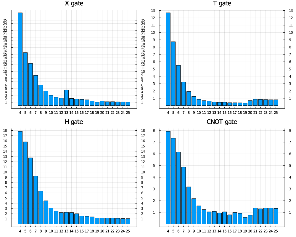
Now let’s see how fast is our ~600 line of code quantum circuit emulator. I don’t intend to go through a complete benchmark here
since the above implementation is generic it will has similar benchmark on different kinds of gates. And there are still plenty
of room to optimize, e.g we can specialize each routine for a known gate, such X gate, H gate to make use of their matrix structure.

The benchmark of multi-threaded routines and CUDA is currently missing since I don’t have access to a
GPU with ComplexF64 support to make the comparison fair. However, this blog post is a simple version of
YaoArrayRegister
in the Yao ecosystem, you can use the benchmark of Yao for reference. Or please also feel free to
benchmark the implementation and play with it in this blog post yourself for sure!

Let me compare this with one of the current best performance simulator qulacs, you should be able
to find relative benchmark comparing qulacs and other software here.
(I’m not comparing with Yao because the implementation is similar to what is implemented in Yao.)

first we clone the benchmark repo

1

git clone https://github.com/Roger-luo/quantum-benchmarks.git

then checkout to the stable release branch release-0.1

1
2
3

cd quantum-benchmarks && git checkout release-0.1
bin/benchmark setup qulacs
bin/benchmark run qulacs

this will prepare us the benchmark data on our machine. then we benchmark our own implementation

1
2
3
4
5
6
7
8
9
10
11
12
13
14
15
16
17
18
19
20
21
22
23
24
25
26
27
28
29
30
31
32

using BenchmarkTools

data = Dict(
    "X" => [],
    "T" => [],
    "H" => [],
    "CNOT" => [],
)

for n in 4:25
    st = rand(ComplexF64, 1<<n)
    t = @benchmark broutine!(r, $([0 1;1 0]), (3, )) setup=(r=copy($st))
    push!(data["X"], minimum(t).time)
end

for n in 4:25
    st = rand(ComplexF64, 1<<n)
    t = @benchmark broutine!(r, $([1 0;0 exp(im * π / 4)]), (3, )) setup=(r=copy($st))
    push!(data["T"], minimum(t).time)
end

for n in 4:25
    st = rand(ComplexF64, 1<<n)
    t = @benchmark broutine!(r, $([1/sqrt(2) 1/sqrt(2); 1/sqrt(2) -1/sqrt(2)]), (3, )) setup=(r=copy($st))
    push!(data["H"], minimum(t).time)
end

for n in 4:25
    st = rand(ComplexF64, 1<<n)
    t = @benchmark broutine!(r, $([0 1;1 0]), (2, ), (3, ), (1, )) setup=(r=copy($st))
    push!(data["X"], minimum(t).time)
end

note: we always use minimum time as a stable estimator for benchmarks

now we plot the benchmark of X, H, T, CNOT in relative time, to see how good our own simulator is comparing to
one of the best Python/C++ based circuit simulator in single thread.

What’s more?

Recall our previous implementation, since we didn’t specify our matrix type or vector type
to be a Vector or other concrete type, and didn’t specify the element type has to be a ComplexF64 either,
this means ANY subtype of AbstractVector, and ANY subtype of Number can be used with the above methods.
Now we can do something interesting, e.g we can automatically get the ability of symbolic calculation by
feeding symbolic number type from SymEngine package or SymbolicUtils package.
Or we can use Dual number to perform forward mode differentiation directly. Or we can estimate error
by using the error numbers from Measurements.

Here is demo of using SymEngine:

1
2
3
4
5
6
7
8
9
10
11
12
13
14
15
16
17
18

using SymEngine

julia> @vars α θ
(α, θ)

julia> st = Basic[1, α, 0, 0]
4-element Array{Basic,1}:
 1
 α
 0
 0

julia> broutine!(st, [exp(-im * θ) 0; 0 exp(im * θ)], (1, ))
4-element Array{Basic,1}:
  exp(-im*θ)
 exp(im*θ)*α
           0
           0

This is only possible when one is able to use generic programming to write
high performance program, which is usually not possible in the two-language solution Python/C++ without implementing one’s own
type system and domain specific language (DSL) compiler, which eventually becomes some efforts that reinventing the wheels.

Conclusion

Getting similar performance or beyond comparing to Python/C++ solution in numerical computation
is easily achievable in pure Julia with much less code. Although, we should wrap some of the overlapping
code into functions and call them as a better practice, we still only use less than 600 lines of code
with copy pasting everywhere.

Moreover, the power of generic programming will unleash our thinking of numerical methods on many different numerical types.

Experienced readers may find there may still rooms for further optimization, e.g we didn’t specialize much common gates yet, and the loop unroll size might not be the perfect size, and may still vary due to the machine.

Last, besides simulating quantum circuits, the above implementation of subspace matrix multiplication is actually a quite common routine happens frequently in tensor contraction (because quantum circuits are one kind of tensor network), thus more promising application can be using these routines for tensor contraction, however, to make these type of operations more efficient, it may require us to implement BLAS level 3 operation in the subspace which is the subspace matrix-matrix multiplication, which can require more tricks and more interesting.

I uploaded the implementation as a gist: https://gist.github.com/Roger-luo/0df73cabf4c91f9854657fdd2ed66767

I wrote a blog post about how to implement your own (operator overloading based) automatic differentiation (AD) in one day (actually 3 hrs) last year. AD looks like magic sometimes, but I’m going to talk about some black magic this time: the source
to source automatic differentiation. I wrote this during JuliaCon 2019 hackthon with help from Mike Innes.
It turns out that writing a blog post takes longer than writing a source to source AD ;-). This is basically just simple version of Zygote.

I wrap this thing as a very simple package here, if you want to look at more detailed implementation: YASSAD.jl.

If you have used operator overloading based AD like PyTorch, Flux/Tracker, AutoGrad, you may find they have some limitations:

• A Tensor type or Variable type provided by the package has to be used for tracing the function calls
• They cannot handle control flows in general, even in some cases, some workarounds can be taken

However, programming without control flow is not programming! And it is usually very annoying to rewrite a lot code with tracked types. If we want to have a framework for Differentiable Programming as what people like Yan LeCun has been proposing, we need to solve these two problems above.

In fact, these problems are quite straight forward to solve in source to source automatic differentiation, since we basically know everything happens. I will implement a very simple source to source AD without handling control flows, you can also check the complete implementation as Zygote.jl.

But before we start, let’s review some basic knowledge.

Basics

The compilation process of Julia language

I will briefly introduce how Julia program is compiled and run in this section:

1. all the code are just strings
2. the Julia parser will parse the strings first to get an Abstract Syntax Tree (AST)
3. some of the nodes in this AST are macros, macros are like compiled time functions on expressions, the compiler will expand the macros. Then we get an expanded version of AST, which do not have any macros. You can inspect the results with @macroexpand.
4. Now, we will lower the AST, get rid of syntax sugars and represent them in Static Single Assignment Form (SSA), you can get it with @code_lowered, and you can modify this process with Julia macros.
5. When function call happens, we use the function signature to dispatch the function to a certain method, and start doing type inference. You can modify this process with @generated functions, and check the results with @code_typed.
6. The compiler will then generate the llvm IR. You can inspect them with @code_llvm
7. After we have llvm IR, Julia will use llvm to generate native code to actually exectute this function.
8. By executing the function, we will meet another function call, so we go back to step 5

I steal a diagram from JuliaCon 2018 to demonstrate this process:

As you can see. Julia is not a static compiled language, and it uses function as boundary of compilation.

SSA Form IR

A complete introduction of SSA can be a book. But to implement your own source
to source AD only require three simple concept:

• all the variable will only be assigned once
• most variable comes from function calls
• all the control flows become branches

If you have read my last post, I believe you have understand what is computation graph, but now let’s look at this diagram again: what is this computation graph exactly?

While doing the automatic differentiation, we represent the process of computation as a diagram. Each node is an operator with a intermediate value. And each operator also have an adjoint operator which will be used in backward pass. Which means each variable
in each node will only be assigned once. This is just a simple version of SSA Form right?

The gradient can be then considered as an adjoint program of the original program. And the only thing we need to do is to generate the adjoint program. In fact, this is often called Wengert list, tape or graph as described in Zygote’s paper: Don’t Unroll Adjoint. Thus we can directly use the SSA form as our computational graph. Moreover, since in Julia the SSA form IR is lowered, it also means we only need to defined a few primitive routines instead of defining a lot operators.

Since the backward pass is just an adjoint of the original program, we can just write it as a closure

1
2
3
4
5
6
7

function forward(::typeof(your_function), xs...)
    # function declaration
    output = # function output
    output, function (Δ)
        # a closure
    end
end

The advantage of defining this as closure is that we can let the compiler itself handle shared variable between the adjoint program
and the original program instead of managing it ourselves (like what we do in my last post). We call these closures pullbacks.

So given a function like the following

1
2
3
4
5

function foo(x)
    a = bar(x)
    b = baz(x)
    return b
end

If we do this manually, we only need to define a forward function

1
2
3
4
5
6
7
8
9

function forward(::typeof(foo), x)
      x1, back1 = forward(baz, x)
      x2, back2 = forward(bar, x1)
      return x2, function (Δ)
         dx1 = back2(Δ)
         dx2 = back1(dx1)
         return dx2
      end
end

In general, an adjoint program without control flow is just applying these pullbacks generated by their forward function in reversed order. But how do we do this automatically? Someone may say: let’s use macros! Err, we can do that. But our goal is to differentiate arbitrary function defined by someone else, so things can be composable. This is not what we want. Instead, we can tweak the IR, the generated functions in Julia can not only return a modified AST from type information, it can also return the IR.

The generated function can be declared with a @generated macro

1
2
3

@generated function foo(a, b, c)
    return :(1 + 1)
end

It looks like a function as well, but the difference is that inside the function, the value of each function argument a, b, c
is their type since we do not have their values during compile time.

In order to manipulate the IR, we need some tools. Fortunately, there are some in IRTools, we will use this package to generate the IR code.

First, we can use @code_ir to get the IR object processed by IRTools. Its type is IR. The difference between the one you get from @code_lowered is that this will not store the argument name, all the variables are represented by numbers, and there are some useful function implemented for this type.

1
2
3
4
5

julia> @code_ir foo(1.0)
1: (%1, %2)
  %3 = (Main.baz)(%2)
  %4 = (Main.bar)(%3)
  return %4

In this form, each line of code is binded to a variable, we call the right hand statement, and left hand variable. You use a dict-like interface to use this object, e.g

1
2
3
4

julia> using IRTools: var

julia> ir[var(3)]
IRTools.Statement(:((Main.baz)(%2)), Any, 1)

It will return a statement object, which stores the expression of this statement, the inferred type (since we are using the IR before type inference, this is Any). For simplicity, we will not use typed IR in this post (since in principal, their implementations are similar). The last number is the line number.

What is the first number 1 in the whole block? It means code block, in SSA form we use this to represent branches, e.g

1
2
3
4
5
6
7
8
9
10
11
12
13
14
15
16
17
18
19

julia> function foo(x)
           if x > 1
               bar(x)
           else
               baz(x)
           end
       end
foo (generic function with 1 method)

julia> @code_ir foo(1.0)
1: (%1, %2)
  %3 = %2 > 1
  br 3 unless %3
2:
  %4 = (Main.bar)(%2)
  return %4
3:
  %5 = (Main.baz)(%2)
  return %5

ifelse is just branch statement in lowered SSA form, and in fact, for loops are similar. Julia’s for loop is just a syntax sugar of iterate function. As long as we can differentiate through br, we will be able to differentiate through control flows.

1
2
3
4
5
6
7
8
9
10
11
12
13
14
15
16
17
18
19
20
21
22
23
24
25
26
27
28

julia> function foo(x)
           for x in 1:10
               bar(x)
           end
           baz(x)
       end
foo (generic function with 1 method)

julia> @code_ir foo(1.0)
1: (%1, %2)
  %3 = 1:10
  %4 = (Base.iterate)(%3)
  %5 = %4 === nothing
  %6 = (Base.not_int)(%5)
  br 3 unless %6
  br 2 (%4)
2: (%7)
  %8 = (Core.getfield)(%7, 1)
  %9 = (Core.getfield)(%7, 2)
  %10 = (Main.bar)(%8)
  %11 = (Base.iterate)(%3, %9)
  %12 = %11 === nothing
  %13 = (Base.not_int)(%12)
  br 3 unless %13
  br 2 (%11)
3:
  %14 = (Main.baz)(%2)
  return %14

So how do we get the IR? In order to get the IR, we need to know which method is dispatched for this generic function. Each generic
function in Julia has a method table, you can use the type signature of the function call to get this method, e.g when you call foo(1.0), Julia will generate Tuple{typeof(foo), Float64} to call the related method. We can get the meta information of this method by providing the IRTools.meta function with this type signature

1
2
3
4
5

julia> IRTools.IR(m)
1: (%1, %2)
  %3 = (Main.baz)(%2)
  %4 = (Main.bar)(%3)
  return %4

And we can manipulate this IR with functions like push!:

1
2
3
4
5
6
7
8
9

julia> push!(ir, :(1+1))
%5

julia> ir
1: (%1, %2)
  %3 = (Main.baz)(%2)
  %4 = (Main.bar)(%3)
  %5 = 1 + 1
  return %4

IRTools will add the variable name for you automatically here. Similarly, we can use insert! to insert a statement before the 4th variable:

1
2
3
4
5
6
7
8
9
10
11

julia> using IRTools: var

julia> insert!(ir, var(4), :(1+1))
%5

julia> ir
1: (%1, %2)
  %3 = (Main.baz)(%2)
  %5 = 1 + 1
  %4 = (Main.bar)(%3)
  return %4

Or we can insert a statement after the 4th variable:

1
2
3
4
5
6
7
8
9
10
11
12

julia> using IRTools: insertafter!

julia> insertafter!(ir, var(4), :(2+2))
%6

julia> ir
1: (%1, %2)
  %3 = (Main.baz)(%2)
  %5 = 1 + 1
  %4 = (Main.bar)(%3)
  %6 = 2 + 2
  return %4

With these tools, we can now do the transformation of forward pass. Our goal is to replace each function call with the function call to forward function and then collect all the pullbacks returned by forward function to generate a closure. But wait! I didn’t mention closure, what is the closure in SSA IR? Let’s consider this later, and implement the transformation of forward part first.

Let’s take a statement and have a look

1
2
3
4
5
6
7
8
9
10
11
12

julia> dump(ir[var(3)])
IRTools.Statement
  expr: Expr
    head: Symbol call
    args: Array{Any}((2,))
      1: GlobalRef
        mod: Module Main
        name: Symbol baz
      2: IRTools.Variable
        id: Int64 2
  type: Any
  line: Int64 1

In fact, we only need to check whether the signature of its expression is call. We can use the Pipe object in IRTools to do the transformation, the transformation results are stored in its member to.

1
2

julia> IRTools.Pipe(ir).to
1: (%1, %2)

Implementation

Forward Transformation

We name this function as register since it has similar functionality as our old register function in my last post. The only difference is: you don’t need to write this register function manually for each operator now! We are going to do this automatically.

Warning: since I’m doing this demo in REPL, I use Main module directly, if you put the code in your own module, replace it with your module name.

1
2
3
4
5
6
7
8
9
10
11
12

function register(ir)
    pr = Pipe(ir)
    argument!(pr, at = 1)
    for (v, st) in pr
        ex = st.expr
        if Meta.isexpr(ex, :call)
            yJ = insert!(pr, v, stmt(xcall(Main, :forward, ex.args...), line = ir[v].line))
            pr[v] = xgetindex(yJ, 1)
        end
    end
    finish(pr)
end

I’ll explain what I do here: first since we are generating the IR for the forward function, we have an extra argument now

1

forward(f, args...)

Thus, I added one argument at the beginning of this function’s IR.

Then, we need to iterate through all the variables and statements, if the statement is a function call then we replace it with the call
to forward function. Remember to keep the line number here, since we still want some error message. Since the returned value of forward is a tuple of actually forward evaluation and the pullback, to get the correct result we need to index this tuple, and replace
the original variable with the new one. The xgetindex here is a convenient function that generates the expression of getindex

1

xgetindex(x, i...) = xcall(Base, :getindex, x, i...)

Let’s see what we get

1
2
3
4
5
6
7

julia> register(ir)
1: (%3, %1, %2)
  %4 = (Main.forward)(Main.baz, %2)
  %5 = (Base.getindex)(%4, 1)
  %6 = (Main.forward)(Main.bar, %5)
  %7 = (Base.getindex)(%6, 1)
  return %7

Nice! We change the function call to forward now!

Now, it’s time to consider the closure problem. Yes, in this lowered form, we don’t have closures. But we can instead store them in a callable object!

1
2
3
4
5

struct Pullback{S, T}
    data::T
end

Pullback{S}(data::T) where {S, T} = Pullback{S, T}(data)

This object will also store the function signature, so when we call pullback, we can look up the IR of the original call to generate the IR of this pullback. The member data here will store a Tuple of all pullbacks with the order of their forward call. In order to construct the Pullback we need the signature of our function call, so we need to revise our implementation as following.

1
2
3
4
5
6
7
8
9
10
11
12
13
14
15
16
17
18

function register(ir, F)
    pr = Pipe(ir)
    pbs = Variable[]
    argument!(pr, at = 1)
    for (v, st) in pr
        ex = st.expr
        if Meta.isexpr(ex, :call)
            yJ = insert!(pr, v, stmt(xcall(Main, :forward, ex.args...), line = ir[v].line))
            pr[v] = xgetindex(yJ, 1)
            J = insertafter!(pr, v, stmt(xgetindex(yJ, 2), line = ir[v].line))
            push!(pbs, substitute(pr, J))
        end
    end
    pr = finish(pr)
    v = push!(pr, xtuple(pbs...))
    pbv = push!(pr, Expr(:call, Pullback{F}, v))
    return pr
end

In order to store the pullbacks, we need to get the pullback from the tuple returned by forward and allocate a list to record all pullbacks.

Here xtuple is similar to xgetindex, it is used to generate the expression of constructing a tuple.

1

xtuple(xs...) = xcall(Core, :tuple, xs...)

Let’s pack the pullback and the original returned value as a tuple together, and return it!

1
2
3
4
5
6
7
8
9
10
11
12
13
14
15
16
17
18
19
20
21

function register(ir, F)
    pr = Pipe(ir)
    pbs = Variable[]
    argument!(pr, at = 1)
    for (v, st) in pr
        ex = st.expr
        if Meta.isexpr(ex, :call)
            yJ = insert!(pr, v, stmt(xcall(Main, :forward, ex.args...), line = ir[v].line))
            pr[v] = xgetindex(yJ, 1)
            J = insertafter!(pr, v, stmt(xgetindex(yJ, 2), line = ir[v].line))
            push!(pbs, substitute(pr, J))
        end
    end
    pr = finish(pr)
    v = push!(pr, xtuple(pbs...))
    pbv = push!(pr, Expr(:call, Pullback{F}, v))
    ret = pr.blocks[end].branches[end].args[1]
    ret = push!(pr, xtuple(ret, pbv))
    pr.blocks[end].branches[end].args[1] = ret
    return pr, pbs
end

The return statement is actually a simple branch, it is the last branch of the last statement of the last code block.

OK, let’s see what we get now

1
2
3
4
5
6
7
8
9
10
11
12

julia> register(ir, Tuple{typeof(foo), Float64})
1: (%3, %1, %2)
  %4 = (Main.forward)(Main.baz, %2)
  %5 = (Base.getindex)(%4, 1)
  %6 = (Base.getindex)(%4, 2)
  %7 = (Main.forward)(Main.bar, %5)
  %8 = (Base.getindex)(%7, 1)
  %9 = (Base.getindex)(%7, 2)
  %10 = (Core.tuple)(%9, %6)
  %11 = (Pullback{Tuple{typeof(foo),Float64},T} where T)(%10)
  %12 = (Core.tuple)(%8, %11)
  return %12

Now let’s implement the forward function

1
2
3
4
5

@generated function forward(f, xs...)
    T = Tuple{f, xs...}
    m = IRTools.meta(T)
    m === nothing && return
end

We will get the meta first, if the meta is nothing, it means this method doesn’t exist, so we just stop here. If we have the meta, then
we can get the IR from it and put it to register

1
2
3
4
5
6

@generated function forward(f, xs...)
    T = Tuple{f, xs...}
    m = IRTools.meta(T)
    m === nothing && return
    frw = register(IR(m), T)
end

However, the object frw has type IR instead of CodeInfo, to generate the CodeInfo for Julia compiler, we need to put argument names back with

1

argnames!(m, Symbol("#self#"), :f, :xs)

And since the second argument of our forward function is a vararg, we need to tag it to let our compiler know, so the compiler will not feed the first function call with a Tuple.

1

frw = varargs!(m, frw, 2)

In the end, our forward function will looks like

1
2
3
4
5
6
7
8
9

@generated function forward(f, xs...)
    T = Tuple{f, xs...}
    m = IRTools.meta(T)
    m === nothing && return
    frw = register(IR(m), T)
    argnames!(m, Symbol("#self#"), :f, :xs)
    frw = varargs!(m, frw, 2)
    return IRTools.update!(m, frw)
end

Let’s see what we got now

1
2
3
4
5
6
7
8
9
10
11
12
13

julia> @code_ir forward(foo, 1.0)
1: (%1, %2, %3)
  %4 = (Base.getfield)(%3, 1)
  %5 = (Main.forward)(Main.baz, %4)
  %6 = (Base.getindex)(%5, 1)
  %7 = (Base.getindex)(%5, 2)
  %8 = (Main.forward)(Main.bar, %6)
  %9 = (Base.getindex)(%8, 1)
  %10 = (Base.getindex)(%8, 2)
  %11 = (Core.tuple)(%10, %7)
  %12 = (Main.Pullback{Tuple{typeof(foo),Float64},T} where T)(%11)
  %13 = (Core.tuple)(%9, %12)
  return %13

If you try to actually run this, there will be some error unfortunately

1
2
3
4
5
6
7
8
9
10

julia> forward(foo, 1.0)
ERROR: MethodError: no method matching getindex(::Nothing, ::Int64)
Stacktrace:
 [1] * at ./float.jl:399 [inlined]
 [2] forward(::typeof(*), ::Float64, ::Float64) at /Users/roger/.julia/dev/YASSAD/src/compiler.jl:0
 [3] baz at ./REPL[4]:1 [inlined]
 [4] forward(::typeof(baz), ::Float64) at /Users/roger/.julia/dev/YASSAD/src/compiler.jl:0
 [5] foo at ./REPL[2]:1 [inlined]
 [6] forward(::typeof(foo), ::Float64) at /Users/roger/.julia/dev/YASSAD/src/compiler.jl:0
 [7] top-level scope at none:0

This is because the forward will be recursively called, which also means we only need to define the inner most (primitive) operators by overloading the forward functions, e.g we can overload the * operator in this case

1
2
3
4

julia> forward(::typeof(*), a::Real, b::Real) = a * b, Δ->(Δ*b, a*Δ)

julia> forward(foo, 1.0)
(1.0, YASSAD.Pullback{.....}

Backward Transformation

But this pullback is not callable yet. Let’s generate the IR for pullback. Similarly, we can define

1
2
3
4
5
6
7
8
9

@generated function (::Pullback{S})(delta) where S
    m = IRTools.meta(S)
    m === nothing && return
    ir = IR(m)
    _, pbs = register(ir, S)
    back = adjoint(ir, pbs)
    argnames!(m, Symbol("#self#"), :delta)
    return IRTools.update!(m, back)
end

Because the backward pass is called separately, we don’t have the forward IR anymore, unfortunately we need to call register again here, but no worries, this will only happen once during compile time. Before we generate the IR for adjoint program, we also need to know which variable has pullback, thus instead of using a list, we need a dict to store this, and return it to pullback. Therefore, we need to revise our register as following

1
2
3
4
5
6
7
8
9
10
11
12
13
14
15
16
17
18
19
20
21

function register(ir, F)
    pr = Pipe(ir)
    pbs = Dict{Variable, Variable}()
    argument!(pr, at = 1)
    for (v, st) in pr
        ex = st.expr
        if Meta.isexpr(ex, :call)
            yJ = insert!(pr, v, stmt(xcall(Main, :forward, ex.args...), line = ir[v].line))
            pr[v] = xgetindex(yJ, 1)
            J = insertafter!(pr, v, stmt(xgetindex(yJ, 2), line = ir[v].line))
            pbs[v] = substitute(pr, J)
        end
    end
    pr = finish(pr)
    v = push!(pr, xtuple(values(pbs)...))
    pbv = push!(pr, Expr(:call, Pullback{F}, v))
    ret = pr.blocks[end].branches[end].args[1]
    ret = push!(pr, xtuple(ret, pbv))
    pr.blocks[end].branches[end].args[1] = ret
    return pr, pbs
end

since the adjoint program has the reversed order with the original IR, we will not use Pipe here, we can create an empty IR object,
and add two argument to it here, one is the Pullback object itself, the other is the input gradient of the backward pass (pullback).

1
2
3

adj = empty(ir)
self = argument!(adj)
delta = argument!(adj)

First, let’s get our pullbacks. The getfield function I call here is the lowered form of syntax sugar . for getting members, this is equivalent to self.data.

1

pullbacks = pushfirst!(adj, xcall(:getfield, self, QuoteNode(:data)))

Then let’s iterate the all the variables in reversed order

1
2
3
4
5
6
7
8
9

vars = keys(ir)
for k in length(vars):-1:1
    v = vars[k]
    ex = ir[v].expr
    if haskey(pbs, v)
        pbv = insertafter!(adj, pullbacks, xcall(:getindex, pullbacks, k))
        g = push!(adj, Expr(:call, pbv, v))
    end
end

if this variable exists in our dict of pullbacks, we get it and call it with this variable. However, there is a problem of this implementation, if one variable has multiple gradient, we need to accumulate them together, thus we need to record these variables’
gradietns as well.

1

grads = Dict()

Then we can implement two method of grad:

1

grad(x, x̄) = push!(get!(grads, x, []), x̄)

Store the gradient x̄ in the list of x in grads.

1

grad(x) = xaccum(adj, get(grads, x, [])...)

Return the accumulated variable of all gradients.

The xaccum is the same as previous xgetindex, but the builtin accumulate function in Julia is defined on arrays, we need one to accumulate variant variables, let’s do it ourselves

1
2
3
4
5
6
7
8
9
10
11
12
13
14

xaccum(ir) = nothing
xaccum(ir, x) = x
xaccum(ir, xs...) = push!(ir, xcall(YASSAD, :accum, xs...))
accum() = nothing
accum(x) = x
accum(x, y) =
  x == nothing ? y :
  y == nothing ? x :
  x + y

accum(x, y, zs...) = accum(accum(x, y), zs...)

accum(x::Tuple, y::Tuple) = accum.(x, y)
accum(x::AbstractArray, y::AbstractArray) = accum.(x, y)

In the end, the pullback will return each input variable’s gradient of the original program. Which means it always has
the same number of gradients as input variables. But our forward function has one extra variable which is the function,
we will return its gradient as well, in most cases, it is nothing, but if it is a closure, or a callable object, it may
not be nothing.

So, in the end, our adjoint function looks like

1
2
3
4
5
6
7
8
9
10
11
12
13
14
15
16
17
18
19
20
21
22
23
24
25
26
27
28
29
30

function adjoint(ir, pbs)
    adj = empty(ir)
    self = argument!(adj)
    delta = argument!(adj)
    pullbacks = pushfirst!(adj, xcall(:getfield, self, QuoteNode(:data)))

    grads = Dict()
    grad(x, x̄) = push!(get!(grads, x, []), x̄)
    grad(x) = xaccum(adj, get(grads, x, [])...)
    grad(last(keys(ir)), delta)

    vars = keys(ir)
    for k in length(vars):-1:1
        v = vars[k]
        ex = ir[v].expr
        if haskey(pbs, v)
            pbv = insertafter!(adj, pullbacks, xcall(:getindex, pullbacks, k))
            g = push!(adj, Expr(:call, pbv, grad(v)))

            for (i, x) in enumerate(ex.args)
                x isa Variable || continue
                grad(x, push!(adj, xgetindex(g, i)))
            end
        end
    end
    gs = [grad(x) for x in arguments(ir)]
    Δ = push!(adj, xtuple(gs...))
    return!(adj, Δ)
    return adj
end

Contextual Dispatch

Reviewing what we just implemented above, we can find we were actually just dispatching functions based on their context instead of
their signature (since the signature is used to dispatch the function themselves). The Julia community actually implements something
more general: the Cassette.jl. Cassette can dispatch function based on a context, and it also contains an implementation of AD as well: Cassette/test. With these mechanism, and the dynamic feature of Julia, we are not only able to implement source to source AD, we can also have

• Sparsity Detection
• SPMD transformation
• Intermediate Variable Optimization
• Debugger: MagneticReadHead
• Unified Interface of CUDAnative

Conclusion

Let’s try this with matrix multiplication + matrix trace, which is the same with what we do in our last post!

Look! we can use the builtin types directly!

1
2
3
4
5
6
7
8
9
10
11
12
13
14
15
16
17
18
19
20
21
22
23
24
25
26
27
28
29

using LinearAlgebra

function forward(::typeof(*), A::Matrix, B::Matrix)
    A * B, function (Δ::Matrix)
        Base.@_inline_meta
        (nothing, Δ * B', A' * Δ)
    end
end

function forward(::typeof(tr), A::Matrix)
    tr(A), function (Δ::Real)
        Base.@_inline_meta
        (nothing, Δ * Matrix(I, size(A)))
    end
end

julia> using LinearAlgebra, BenchmarkTools

julia> mul_tr(A::Matrix, B::Matrix) = tr(A * B)
mul_tr (generic function with 1 method)

julia> A, B = rand(30, 30), rand(30, 30);

julia> mul_tr(A, B)
216.7247235502547

julia> z, back = forward(mul_tr, A, B)；

julia> julia> back(1);

The performance is similar to the manual implementation as well (in fact it should be the same)

The manual version is:

1
2
3
4
5
6
7
8
9
10
11
12

julia> @benchmark bench_tr_mul_base($(rand(30, 30)), $(rand(30, 30)))
BenchmarkTools.Trial: 
  memory estimate:  28.78 KiB
  allocs estimate:  5
  --------------
  minimum time:     10.696 μs (0.00% GC)
  median time:      13.204 μs (0.00% GC)
  mean time:        24.075 μs (43.31% GC)
  maximum time:     62.964 ms (99.97% GC)
  --------------
  samples:          10000
  evals/sample:     1